3. Tutorial

This tutorial will guide you through a typical PyBN application. Familiarity with Python is assumed, so if you are new to Python, books such as [Lutz2007] or [Langtangen2009] are the place to start. Plenty of online documentation can also be found on the Python documentation page.

The tutorial is based on the “Car Start Problem” from the book “Bayesian Networks and Decision Graphs” [Jensen2007]

Warning

A (good) d-separation algorithm is missing at the moment! So the order of the nodes and arcs are very important for the (correct) results.

3.1. Car Start Problem

The following is an example of the type of reasoning that humans do daily.

“In the morning, my car will not start. I can hear the starter turn, but nothing happens. There may be several reasons for my problem. I can hear the starter roll, so there must be power from the battery. Therefore, the most probable causes are that the fuel has been stolen overnight or that the spark plugs are dirty. It may also be due to dirt in the carburetor, a loose connection in the ignition system, or something more serious. To find out, I first look at the fuel meter. It shows half full, so I decide to clean the spark plugs.”

To have a computer do the same kind of reasoning, we need answers to questions such as, “What made me conclude that among the probable causes “stolen fuel”, and “dirty spark plugs” are the two most-probable causes?” or “What made me decide to look at the fuel meter, and how can an observation concerning fuel make me conclude on the seemingly unrelated spark plugs?”

To be more precise, we need ways of representing the problem and ways of performing inference in this representation such that a computer can simulate this kind of reasoning and perhaps do it better and faster than humans.

3.1.1. A Causal Perspective on the Car Start Problem

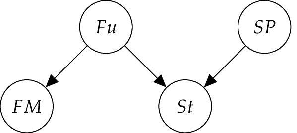
To simplify the situation, assume that we have the events {yes, no} for Fuel? (\(Fu\)), {yes, no} for Clean Spark Plugs? (\(SP\)), {full, half , empty} for Fuel Meter (\(FM\)), and {yes, no} for Start? (\(St\)). In other words, the events are clustered around variables, each with a set of outcomes, also called states. We know that the state of Fuel? and the state of Clean Spark Plugs? have a causal impact on the state of Start?. Also, the state of Fuel? has an impact on the state of Fuel Meter Standing. This is represented by the graph in the Figure below.

For the quantitative modeling, we need the probability assessments \(P (Fu)\), \(P (SP)\), \(P (St | Fu, SP)\), \(P (FM | Fu)\). To avoid having to deal with numbers that are too small, let \(P (Fu) = (0.98, 0.02)\) and \(P (SP) = (0.96, 0.04)\). The remaining tables are given in the Tables below. Note that the table for \(P (FM | Fu)\) reflects the fact that the fuel meter may be malfunctioning, and the table for \(P (St | Fu, SP)\) leaves room for causes other than no fuel and dirty spark plugs by assigning \(P (St = no | Fu = yes, SP = yes) > 0\).

Table \(P (FM | Fu)\):

\(Fu\)	yes	no
full	0.39	0.001
half	0.60	0.001
empty	0.01	0.998

Table \(P (St | Fu, SP)\):

\(Fu\)	yes	yes	no	no
\(SP\)	yes	no	yes	no
yes	0.99	0.01	0	0
no	0.01	0.99	1	1

3.1.2. Let’s model

Before we start with the modeling, we have to import the pybn package. Therefore are two different methods available:

In case 1 we load pybn like a normal library:

import pybn

here we must write for each command pybn.my_command(). A much nicer way to load the package is case 2:

# import pybn library
from pybn import *

here, we import all available objects from pybn.

The first step is the initialization of the network.

# Create a Network
net = Network('CarProblem')

Now the nodes for the Bayesian Network can be created.

# Create Node 'Fuel'
Fu = Node('Fu')

This node should have two states {yes,no}.

# Setting number (and name) of outcomes
Fu.addOutcome('yes')
Fu.addOutcome('no')

The number and name of the outcomes belongs to the definition of the node. We can (and must) define them before any useful inference can be made on the network. Following the same procedure for the node \(SP\), we create a new node and let it have three states:

# Create node 'Clean Spark Plugs'
SP = Node('SP')

# Setting number (and name) of outcomes
SP.addOutcomes(['yes','no'])

Here we created the outcomes with one command, instead of declare each state. In the same way we can define the two other nodes form the network:

# Create node 'Start'
St = Node('St')

# Setting number (and name) of outcomes
St.addOutcomes(['yes','no'])

# Create node 'Fuel Meter Standing'
FM = Node('FM')

# Setting number (and name) of outcomes
FM.addOutcomes(['full','half','empty'])

Now, we can add an arcs from the parent nodes to there children to represent the conditional dependence.

# Add arc from 'Fuel' to 'Start'
arc_Fu_St = Arc(Fu,St)

# Add arc from 'Clean Spark Plugs' to 'Start'
arc_SP_St = Arc(SP,St)

# Add arc from 'Fuel' to 'Fuel Meter Standing'
arc_Fu_FM = Arc(Fu,FM)

Now we need to fill in the distribution of the nodes. We know that the node \(Fu\) and \(SP\) have two states and no parents, so we just need two numbers that represent the probability of each of the states coming true.

# Conditional distribution for node 'Fuel'
Fu.setProbabilities([0.98,0.02])

# Conditional distribution for node 'Clean Spark Plugs'
SP.setProbabilities([0.96,0.04])

Now we have to fill the distribution of the node FM conditioned on the node \(Fu\). Definition matrix in this case, will have two dimensions: one for the states of the parent (\(Fu\)) and one for the states of the child (\(FM\)).

If you not sure about the size of the matrix, you can check the size with FM.getTableSize().

The order of these probabilities is given by considering the state of the first parent of the node as the most significant (thinking of the coordinates in terms of bits) coordinate, then the second parent, then the third (and so on), and finally considering the coordinate of the node itself as the least significant one.:

# Conditional distribution for node 'Fuel Meter Standing'
FM.setProbabilities([0.39, 0.60, 0.01, 0.001, 0.001, 0.998])

In the same way the probabilities for the node St can be defined. Here the node has two parents (\(Fu,SP\)). Since we defined the arc from \(Fu\) to \(St\) before we defined the arc from \(SP\) to \(St\), the probabilities are ordered dependent on \(Fu\) (see Table \(P (St | Fu, SP)\)).:

# Conditional distribution for node 'Start'
St.setProbabilities([0.99, 0.01, 0.01, 0.99, 0.0, 1.0, 0.0, 1.0])

After the network has been created we make it more spatially organized and change a few visual nodes’ attributes.

# Changing the nodes spacial and visual attributes:
Fu.setNodePosition(100,10)

SP.setNodePosition(300,10)

FM.setNodePosition(0,150)
FM.setInteriorColor('cc99ff')

St.setNodePosition(200,150)
St.setInteriorColor('ff0000')

Finally we have to add the nodes to the network.

# Add notes to network
net.addNodes([Fu,SP,St,FM])

Now we can store the network in a file called “CarProblem.xdsl” so we can retrieve it with the program GeNIe. The format of the file will be XDSL. If no file name is chosen, the network name will be used.

# Write file
net.writeFile('CarProblem.xdsl')

The generated network will look like the Figure below, if we do not observe evidence.

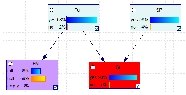
In order to get this result with pybn, the beliefs of the network has to be computed.:

# Compute the beliefs for the network
net.computeBeliefs()

After this step, the beliefs for each node can be printed or used for other calculations.:

# Print the results for each node
print 'Fu', Fu.getBeliefs()
print 'SP', SP.getBeliefs()
print 'St', St.getBeliefs()
print 'FM', FM.getBeliefs()

The result of this calculation will look like this:

Fu [ 0.98  0.02]
SP [ 0.96  0.04]
St [ 0.931784  0.068216]
FM [ 0.38222  0.58802  0.02976]

which is equal to the results computed with GeNIe.

What happens when we observe the car does not start (\(St = no\))? To implement this observation, an evidence for \(St\) must be set. This means that before doing any calculations, we have to enter this evidence into the network.:

# Set evidence
net.setEvidence('St',2)

where 2 denotes the second stage, here no. After this step, the beliefs can be computed again and we get following results:

Fu [ 0.70681365  0.29318635]
SP [ 0.41937375  0.58062625]
St [ 0.  1.]
FM [ 0.27595051  0.42438138  0.29966811]

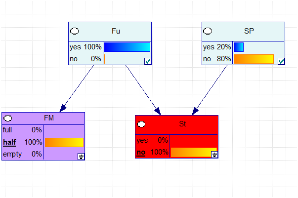
Next, we get the information that \(FM = half\), and the context for calculation is limited to the part with \(FM = half\) and \(St = no\).

# Set evidence
net.setEvidence('FM',2)
net.setEvidence('St',2)

The numbers are given by:

Fu [ 0.99930914  6.90855832e-04]
SP [ 0.19565037  0.80434963]
St [ 0.  1.]
FM [ 0.  1.  0.]

Warning

A (good) d-separation algorithm is missing at the moment! So the order of the nodes and arcs are very important for the (correct) results.

3.2. Finally...

This was a short introduction how to use pybn. The tutorial above is also available on GitHub under example.py.

If you like to learn more about GeNIe visit http://genie.sis.pitt.edu/

Let’s have fun ;)