4. Theoretical Background

4.1. Bayesian Networks

In this section graphical models (GMs), which are the basic graphical feature for Bayesian networks (BNs), will be introduced. [Jensen2007] This theory is implemented in the Python library, Python Bayesian Networks (PyBN).

4.1.1. Graphical Notation and Terminology

Graphical models (GMs) are tools used to visually illustrate and work with conditional independence (CI) among variables in given problems. [Stephenson2000] In particular, a graph consists of a set \(V\) vertices (or nodes) and a set \(E\) of edges (or links ). The vertices correspond to random variables and the edges will denote a certain relationship between two variables. [Pearl2000]

(1)\[ G := \text{graph}~ G = (V,E)\]

With \(V = \{{X}_1,{X}_2,\dots,{X}_n\}\) and \(E = \{({X}_i,{X}_j):i \neq j\}\).

A pair of nodes \(X_i , X_j\) can be connected by a direct edge \(X_i \to X_j\) or an undirected edge \(X_i - X_j\) . A graph is called directed graph if all edges are either \(X_i \to X_j\) or \(X_i \leftarrow X_j\) and called undirected graph if all edges are \(X_i - X_j\) . [Koller2009]

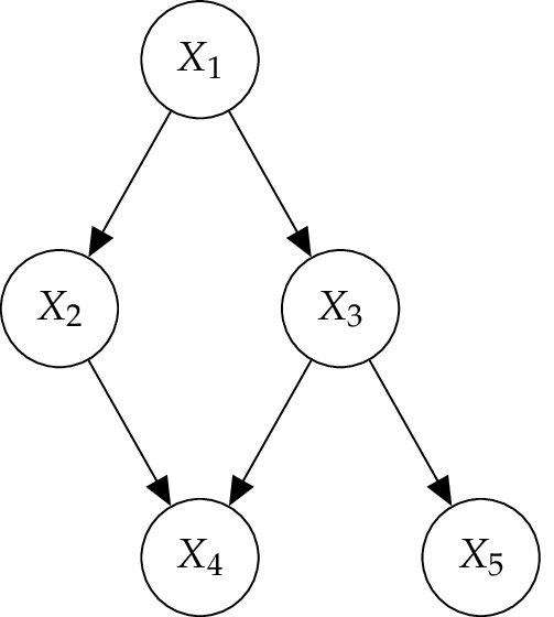
Two variables connected by an edge are called adjacent. A path consists of a series of nodes, where each one is connected to the previous one by an edge. If a path in a graph is a sequence of edges in order that each edge has a directionality going in the same direction, then it is called directed path. For example, \(X_1 \to X_2 \to X_4\) in the Figure above. A directed graph may include direct cycles when a direct part starts and ends at the same node, for instance \(X \to Y \to X\), but this includes no self-loops (\(X \to X\)). A graph that contains no directed cycles is called acyclic, whereas a graph that is directed and acyclic is called directed acyclic graph (DAG) [Pearl2000]. This kind of graph is one of the central concepts which underlies Bayesian networks. [Koller2009]

To denote the relationships in a graph, the terminology of kinship is used. A parent to child relationship in a directed graph occurs in case there is an edge from \(X_1 \to X_2\) . \(X_1\) is called the parent of \(X_2\) and \(X_2\) the child of \(X_1\). If \(X_4\) is a child of \(X_2\) than \(X_1\) is its ancestor and \(X_4\) is \(X_1\) descendant. A family is the set of vertices composed of \(X\) and the parents of \(X_1\); for example, { \(X_2,X_3,X_4\)} in the Figure. The term adjacent (or neighbor) is used to describe the relationship between two nodes connected in an undirected graph. [Stephenson2000]

Furthermore, the notation of a forest is used to define some properties of a directed graph. So a forest is a DAG where each node has either one parent or none at all. A tree is a forest where only one node, called the root, has no parent. However, a node without any parents is called leaf. [Murphy2012]

4.2. Sturcture of Bayesian Networks

Formally BNs are DAG in which each node represents a random variable, or uncertain quantity, which can take on two or more possible values. The edges signify the existence of direct causal influences between linked variables. The strengths of these influences are quantified by conditional probabilities.

In other words, each variable \(X_i\) is a stochastic function of its parents, denoted by \(P( X_i | \text{pa}( X_i ))\). It is called conditional probability distribution (CPD), when \(\text{pa}( X_i )\) is the parent set of a variable \(X_i\). The conjunction of these local estimates specifies a complete and consistent global model (joint probability distribution) on the basis of which all probability queries can be answered. A representing joint probability distribution for all variables is expressed by the chain rule for Bayesian networks [Pearl1988]

Note

[Chain Rule for Bayesian Networks]

Let \(G\) be a DAG over the variables \(V = (X_1 , \dots , X_n )\). Then \(G\) specifies a unique joint probability distribution \(P( X_1 , \dots , X_n )\) given by the product of all CPDs

(2)\[ P(X_1,\dots,X_n) = \prod_{i=1}^n P(X_i|\text{pa}(X_i))\]

This process is called factorization and the individual factors \(\text{pa}( X_i )\) are called CPDs or local probabilistic models. [Koller2009] This properties are used to define a Bayesian network in a formal way.

Note

[Bayesian Network]

A Bayesian Network \(B\) is a tuple \(B = (G , P)\), where \(G = (V , E )\) is a DAG, each node \(X_i \in V\) corresponds to a random variable and \(P\) is a set of CPDs associated with \(G\)’s nodes. The Bayesian Network \(B\) defines the joint probability distribution \(P_B ( X_1 , \dots , X_n )\) according to Equation (2).

For example, is the joint probability distribution corresponding to the network in the Figure above given by

(3)\[ P(X_1,X_2,X_3,X_4,X_5)=P(X_1)P(X_2|X_1)P(X_3|X_1)P(X_4|X_2,X_3)P(X_5|X_3)\]

This structure of a BN can be used to determine the marginal probability or likelihood of each node holding on of its state. This procedure is called marginalisation.

4.3. Evidence

A major advantage of BNs comes by calculating new probabilities, for example, if new information is observed. The effects of the observation are propagated throughout the network and in every propagation step the probabilities of a different node are updated.

New information in a BN are denoted as evidence and defined by a subset \(E\) of random variables in the model and an instantiation \(e\) to these variables.

The task is to compute \(P( X | E = e)\), the posterior probability distribution over the values \(x\) of \(X\), conditioned on the fact that \(E = e\) . This expression can also be viewed as the marginal over \(X\) in the distribution that obtains by conditioning on \(e\). [Koller2009]

Note

Let \(B\) be a Bayesian network over the variables \(V = ( X_1 , \dots , X_n )\) and \(e = (e_1 , \dots , e_m )\) some observations. Then

(4)\[ P(V,e)=\prod_{X\in V}P(X|\text{pa}(X))\cdot\prod_{i=1}^m e_i\]

and for \(X \in V\) follows

(5)\[ P(X|e)=\frac{\sum_{V\backslash X} P(V,e)}{P e}\]

If \(X_1\) and \(X_2\) are d-separated in a BN with evidence \(E = e\) entered, then \(P( X_1 | X_2 , e) = P( X_1 |e)\), this means that \(X_1\) and \(X_2\) are conditional independent given \(E\), denoted \(P ( X_1 \perp X_2 | E)\). [Pearl1988]

4.4. Network Models

At the core of any graphical model is a set of conditional independence assumptions. The aim is to understand when an independence \(( X_1 \perp X_2 | X_3 )\) can be guaranteed. In other words, is it possible that \(X_1\) can influence \(X_2\) given \(X_3\)? [Koller2009]

Deriving these independencies for DAGs is not always easy because of the need to respect the orientation of the directed edges. [Murphy2012] However, a separability criterion, which takes the directionality of the edges in the graph into consideration, is called d-separation. [Pearl1988]

Note

[d-separation]

If \(X_1\) , \(X_2\) and \(X_3\) are three subsets of nodes in a DAG \(G\), then \(X_1\) and \(X_2\) are d-separated given \(X_3\), denoted \(\text{d-sep}_G ( X_1 ; X_2 | X_3 )\), if there is no path between a node \(X_1\) and a node \(X_2\) along with the following two conditions hold:

1. the connection is serial of diverging and the state of \(X_3\) is observed, or
2. the connection is converging and neither the state of \(X_3\) nor the state of any descendant of \(X_3\) is observed.

If a path satisfies the d-separation condition above, it is said to be active, otherwise it is said to be blocked by \(X_3\).

Networks are categorized according to their configuration. The underlying concept can be illustrated by three simple graphs and thereby conditional independencies can be implemented. [Pernkopf2013]

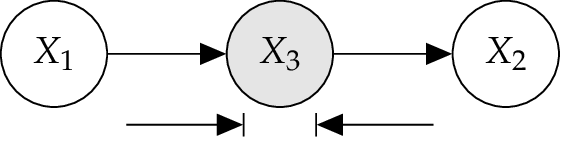
4.4.1. Serial Connection

The BN illustrated in Figure below is a so called serial connection. Here \(X_1\) has an influence on \(X_3\), which in turn has an influence on \(X_2\) . Evidence about \(X_1\) will influence the certainty of \(X_3\), which influences the certainty of \(X_2\), and vice versa by observing \(X_2\). However, if the state of \(X_3\) is known, then the path is blocked and \(X_1\) and \(X_2\) become independent. Now \(X_1\) and \(X_2\) are d-separated given \(X_3\). [Jensen2007]

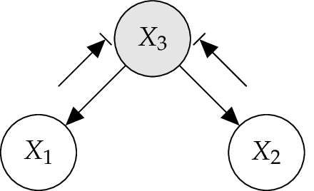
4.4.2. Diverging Connection

In the Figure below, a so called diverging connection for a BN is illustrated. Here influence can pass between all the children of \(X_3\) , unless the state of \(X_3\) is known. When \(X_3\) is observed, then variables \(X_1\) and \(X_2\) are conditional independent given \(X_3\), while, when \(X_3\) is not observed they are dependent in general. [Jensen2007]

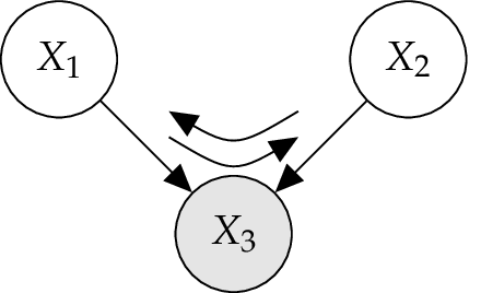
4.4.3. Converging Connection

A converging connection, illustrated in the Figure below, is more sophisticated than the two previous cases. As far nothing is known about \(X_3\) except what may be inferred from knowledge of its parents \(X_1\) and \(X_2\), the parents are independent. This means that an observation of one parent cannot influence the certainties of the other. However, if anything is known about the common child \(X_3\), then the information on one possible cause may tell something about the other cause. [Jensen2007]

In other words, variables which are marginally independent become conditional dependent when a third variable is observed. [Jordan2007]

Note

This important effect is known as explaining away or Berkson’s paradox.

4.5. Dynamic Bayesian Networks

A dynamic Bayesian network (DBN) is just another way to represent stochastic processes using a DAG. To model domains that evolve over time, the system state represents the system at time \(t\) and is an assignment of some set of random variables \(V\). Thereby the random variable \(X_i\) itself is instantiated at different points in time \(t\), represented by \(X_i^t\) and called template variable. To simplify the problem, the timeline is discretized into a set of time slices with a predetermined time interval \(\Delta\). This leads to a set of random variables in form of \(V^0 , V^1 , \dots , V^t , \dots , V^T\) with a joint probability distribution \(P(V^0 , V^1 , \dots , V^t , \dots , V^T )\) over the time \(T\), abbreviated by \(P(V^{0:T} )\). This distribution can be reparameterized. [Koller2009]

(6)\[ P(V^{0:T}) = \prod_{t=0}^{T-1} P(V^{t+1}|V^{0:t})\]

This is the product of conditional distributions, for the variables in each time slice are given by the previous ones.

Note

[Markov assumption]

If the present is known, then the past has no influence on the future.

(7)\[ (V^{t+1} \perp V^{0:(t+1)}|V^{t})\]

This Markov assumption allows to define a compact representation of a DBN:

(8)\[ P(V^{0},\dots,V^{T}) = \prod_{t=0}^{T-1} P(V^{t+1}|V^{t})\]